
Use-case – Diagnosing an automotive engine
This use-case is taken from the conference paper
E. Frisk, M. Krysander, and D. Jung “A Toolbox for Analysis and Design of Model Based Diagnosis Systems for Large Scale Models”, IFAC World Congress, Toulouse, France, 2017.
where the interested reader can find more complete explanations and a full set of references for explainations to used concepts and methods.
This use-case is presented using the Matlab toolbox, but all commands in the use-case have direct counterparts in the Python toolbox.
Outline
- Introduction
- Modelling
- Diagnosability Analysis
- Residual Generator Analysis and Design
- Evaluation on Test Cell Measurements
Introduction
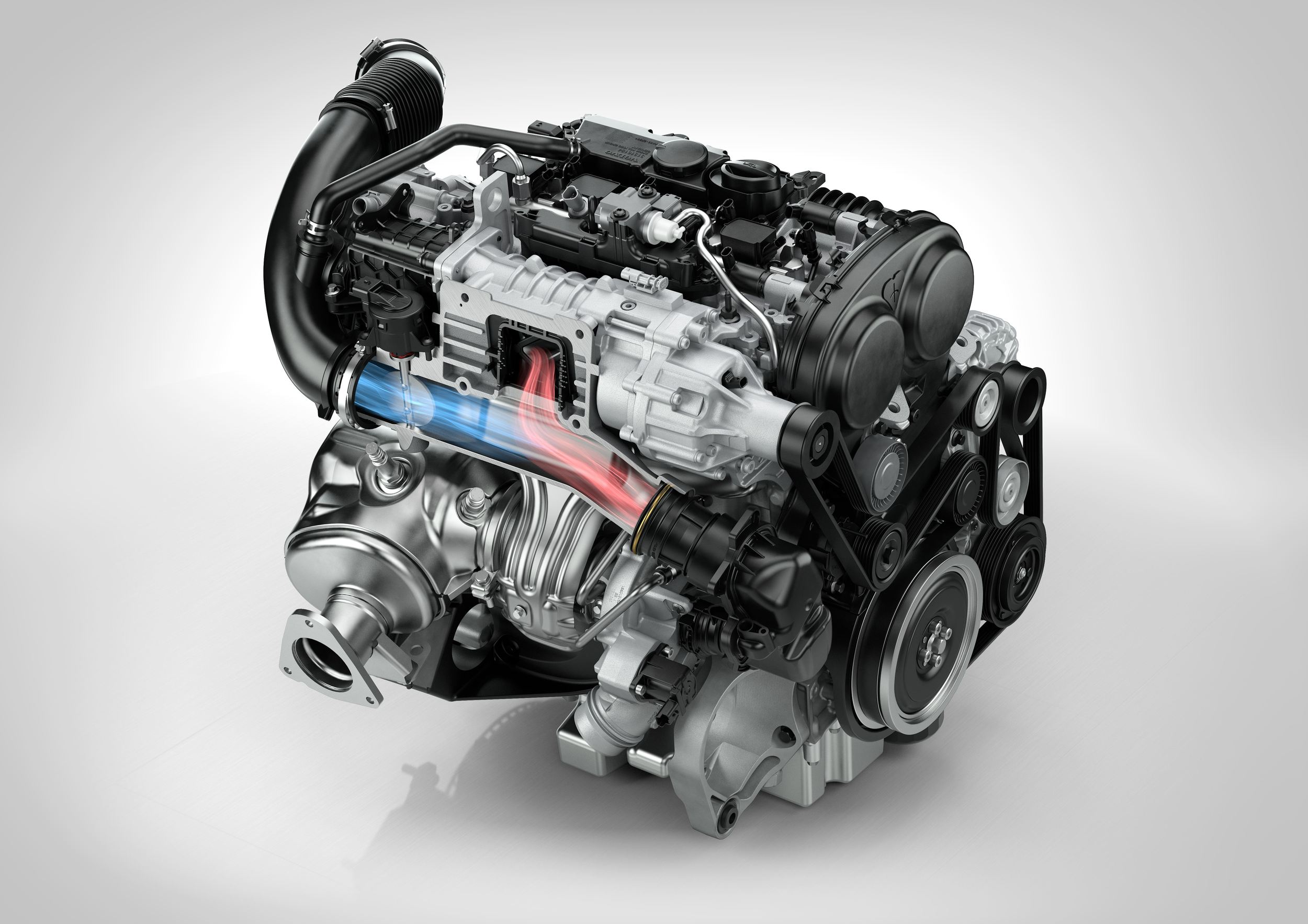 The air-path of an automotive gasoline engine is important for
understanding how much fuel to inject, how to keep combustion emissions low,
protect exhaust catalysts, and optimize efficiency. This system is not only
industrially relevant, it is also an interesting system for academic basic
research due to its complexity, its highly interconnected subsystems due to turbocharging, and
challenging to model accurately. The model used here is based on a control oriented model of the air-path
consisting of pressure dynamics that describe flows and thermodynamic relations to
describe temperatures and heat flows. The model has 94 equations and
14 states. The model is highly non-linear, has
external, mapped, functions implemented as lookup-tables, and hybrid
mode-switching statements (if-statements).
The air-path of an automotive gasoline engine is important for
understanding how much fuel to inject, how to keep combustion emissions low,
protect exhaust catalysts, and optimize efficiency. This system is not only
industrially relevant, it is also an interesting system for academic basic
research due to its complexity, its highly interconnected subsystems due to turbocharging, and
challenging to model accurately. The model used here is based on a control oriented model of the air-path
consisting of pressure dynamics that describe flows and thermodynamic relations to
describe temperatures and heat flows. The model has 94 equations and
14 states. The model is highly non-linear, has
external, mapped, functions implemented as lookup-tables, and hybrid
mode-switching statements (if-statements).
The measurements/control outputs used, in total 10, are: pressure sensors (throttle, intake manifold, ambient), temperature sensors (throttle, ambient), intake air mass flow, engine speed, throttle position, waste-gate position, and commanded amount of injected fuel. The considered faults, in total 11, are: Clogging of the air filter, leakages (before compressor, after throttle, before intercooler), stuck intake valve, increased turbine friction, sensors (throttle position, air mass flow, intake manifold pressure, pressure before throttle, temperature before throttle)
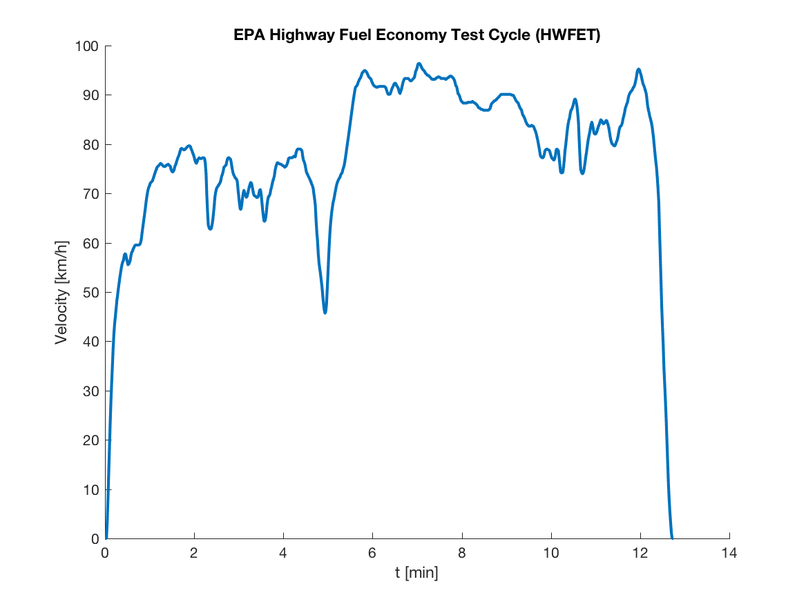 Measurement data is obtained in an engine test cell at Vehicular Systems.
The engine, a standard production engine, is equipped with a development control system
and subjected to load conditions corresponding to a car driving the EPA Highway Fuel Economy Test Cycle.
Engine operation is thus transient, although not violently so, and correct handling
of dynamic engine behavior in the diagnosis system is essential. The objective is then to,
during normal operation, detect and isolate the faults with a given false alarm probability and
optimize detection performance.
Measurement data is obtained in an engine test cell at Vehicular Systems.
The engine, a standard production engine, is equipped with a development control system
and subjected to load conditions corresponding to a car driving the EPA Highway Fuel Economy Test Cycle.
Engine operation is thus transient, although not violently so, and correct handling
of dynamic engine behavior in the diagnosis system is essential. The objective is then to,
during normal operation, detect and isolate the faults with a given false alarm probability and
optimize detection performance.
Modelling
The model is a differential-algebraic (DAE) model, based on the model developed in Eriksson, L. (2007). Modeling and control of turbocharged SI and DI engines. Oil & Gas Science and Technology - Rev. IFP, 62(4), 523–538.
The model-object is created by a statement
m = DiagnosisModel(modelDef)where the struct modelDef is a model definition containing the fields
modelDef.x- cell array of names of unknown variablesmodelDef.f- cell array of names of fault variablesmodelDef.z- cell array of names of known variablesmodelDef.parameters- cell array of parameter namesmodelDef.rels- cell array with model equations
In addition, the model relations/equations are written directly as
symbolic expressions. For example, a restriction model using an
external function W_af_fun, a control volume with a mass
state m_im and a temperature state T_im, and a
measurement equation for the air mass flow W_af can be written
as
%% Declare model equations
modelDef.rels = {
   ...
   % Air filter restriction:
   W_af == W_af_fun(p_amb,p_af,plin_af,
      H_af,T_amb)+fp_af

   % Control volume intake manifold:
   p_im == m_im*R_air*T_im/V_im
   dmdt_im == (W_th - W_ac) + fw_th
   dTdt_im == (W_th*cv_air*(T_imcr-T_im)+R_air*
      (T_imcr*W_th-T_im*W_ac))/(m_im*cv_air)

   % Measurement signals:
   y_W_af == W_af + fyw_af % Air mass flow
   ...
}
The toolbox supports only structural models, but here models with symbolic
model equations is used since the objective of the use case is to go
from model to generating code for residual generators and then expressions
for the model equations are needed. When the modelDef structure has been defined and
the model object has been created it is time to explore the
model. Basic model information is obtained using the Lint class method
>> model.Lint()
Model: Engine model
Type: Symbolic, dynamic
Variables and equations
90 unknown variables
10 known variables
11 fault variables
94 equations, including 14 differential
constraints
Degree of redundancy: 4
Degree of redundancy of MTES set: 1
Model validation finished with 0 errors and
0 warnings.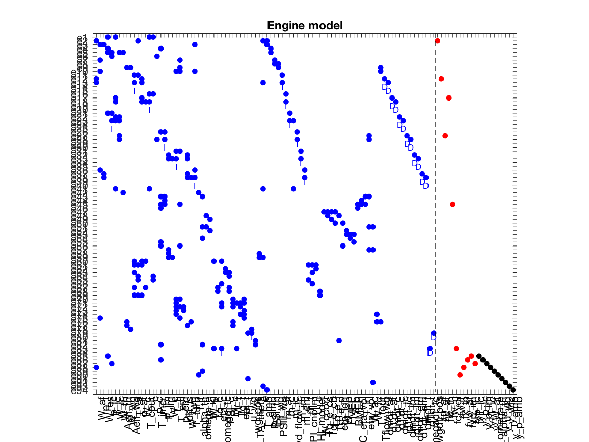 The model structure, i.e., which variables that appear in which constraints, are
extensively used by the methods implemented in the toolbox. This model structure
is automatically inferred from the model equations and the
The model structure, i.e., which variables that appear in which constraints, are
extensively used by the methods implemented in the toolbox. This model structure
is automatically inferred from the model equations and the PlotModel class method can
be used to visualize the model structure. It shows the equations on the vertical axis
and the variables on the horizontal axis. A dot represent that a
variable appears in the corresponding equation. Blue, red, and black
dots represent unknown, fault, and known variables respectively.
>> model.PlotModel()Diagnosability Analysis
Now, with a defined model there are many diagnosis analyses that can be performed on the model structure only. For example, it is possible to find out if the model contains enough redundancy to detect and isolate faults, i.e., answer diagnosability questions like
“Can I detect this fault?” or “Can I isolate this fault from that fault?” or “What isolation performance is possible using only direct application of state-observers?”
Such non-trivial questions can be answered using structural techniques giving best-case results.
A canonical decomposition
A key tool in structural analysis for fault diagnosis is the
Dulmage-Mendelsohn decomposition.
To plot the decomposition, extended with fault variables and equivalence classes
as described in (Krysander and Frisk, 2008),
is computed using the PlotDM class method
model.PlotDM('eqclass', true, 'fault', true)which results in the plot
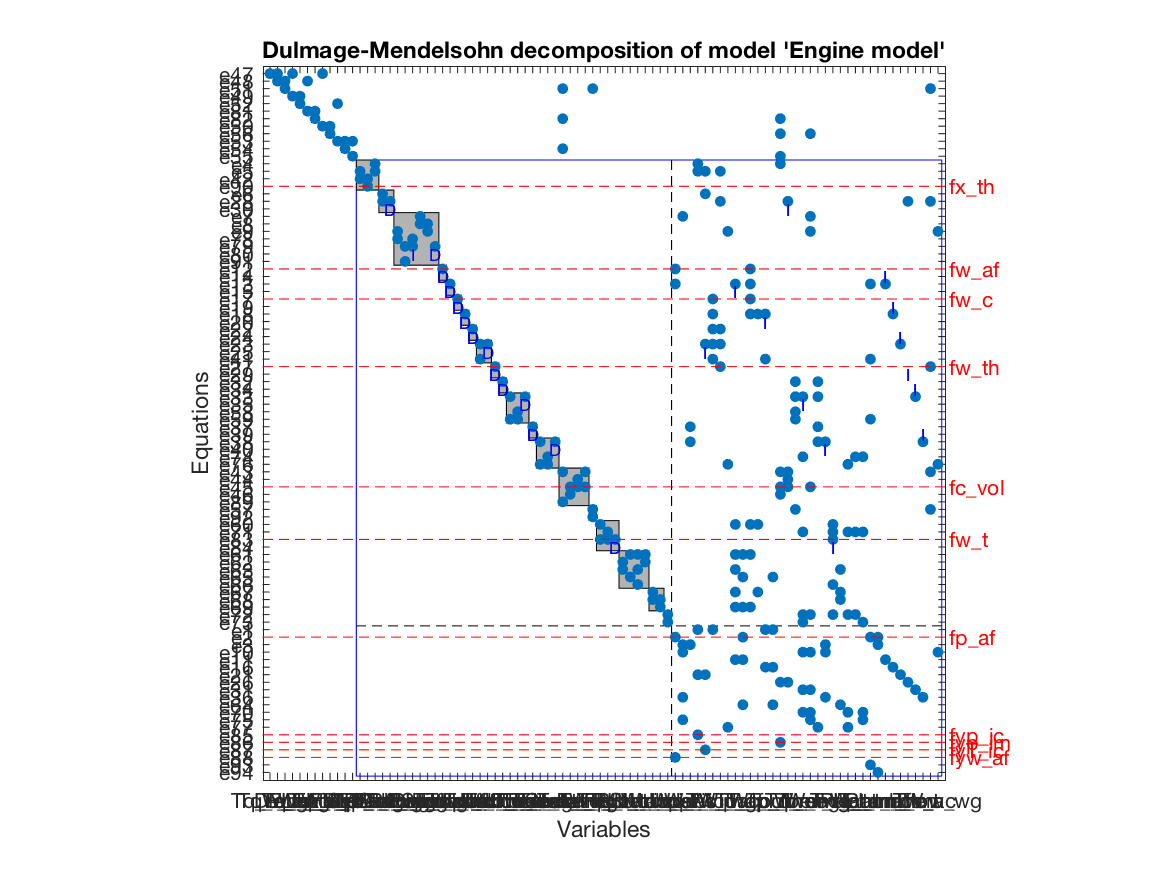
It is a Dulmage-Mendelsohn decomposition with an additional canonical decomposition of the overdetermined part. The overdetermined part is marked with a blue rectangle and faults entering in equations contained in the overdetermined part are structurally detectable. The set of equations in the overdetermined part is partitioned into equivalence classes, indicated by gray shaded rectangles in the figure, with the property that all faults appearing in the same equivalence class is not structurally isolable from each other.
Fault isolability Matrices
Although the canonical form is informative, it contains
a lot of details. Another form of illustrating single fault
isolability performance is the isolability matrix computed using
the class method IsolabilityAnalysis as
model.IsolabilityAnalysis()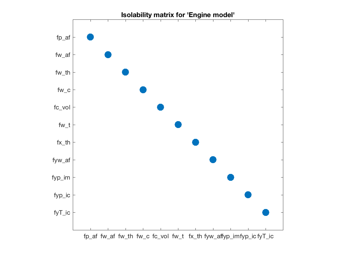 A dot in position (i,j) indicates fault j will be a diagnosis if
fault i is the present fault. Thus a diagonal matrix represents full
single fault isolability, i.e., all single faults are uniquely
structurally isolable in the engine model.
A dot in position (i,j) indicates fault j will be a diagnosis if
fault i is the present fault. Thus a diagonal matrix represents full
single fault isolability, i.e., all single faults are uniquely
structurally isolable in the engine model.
Low structural index is an interesting class of models since, for example, for low-index models established techniques like state-observers and Extended Kalman Filters can be directly applied while this is not true for high-index models. The isolability of faults when only using low-index approaches can be computed by
model.IsolabilityAnalysis('causality','int')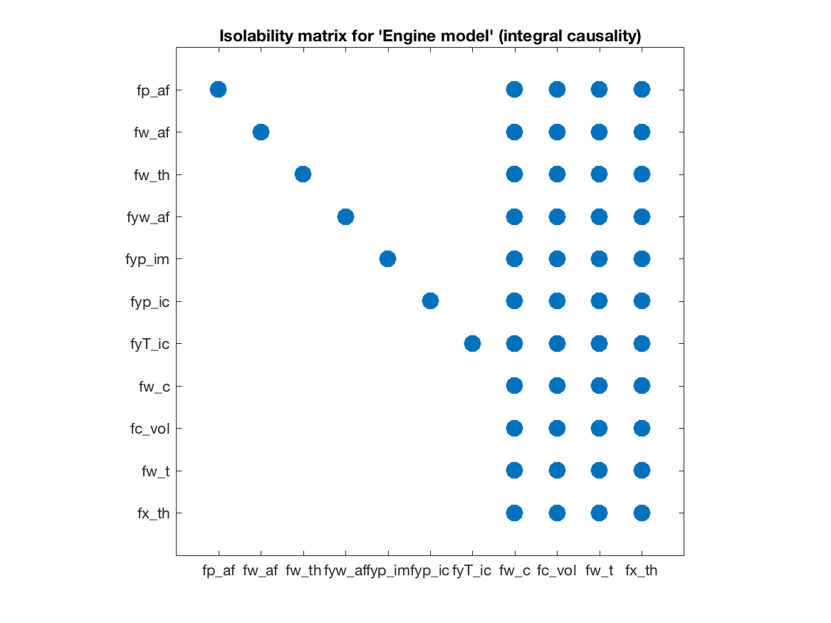 The isolability matrix shows how the fault isolability performance
degrades, which is expected, if the residual generation techniques are
limited to pure integration based methods. These isolability matrices gives a
direct way to early evaluate possible isolation performance of the model
and with the given measurements. Of course, these are structural results meaning
that even if the isolability matrix indicate that all faults are uniquely
isolable, it is not certain that this is realizable in the real application with
a required detection and false-alarm probabilities. But is gives an important
first indication on what is possible.
The isolability matrix shows how the fault isolability performance
degrades, which is expected, if the residual generation techniques are
limited to pure integration based methods. These isolability matrices gives a
direct way to early evaluate possible isolation performance of the model
and with the given measurements. Of course, these are structural results meaning
that even if the isolability matrix indicate that all faults are uniquely
isolable, it is not certain that this is realizable in the real application with
a required detection and false-alarm probabilities. But is gives an important
first indication on what is possible.
Residual Generator Analysis and Design
One successful approach to residual generation is to find testable
sub-models and then, based on such sub-models, design residual
generators. The first step is then to make a complete search for
testable sub-models, here Minimally Structurally Overdetermined (MSO)
set of equations. This step is based only on the
structure of the model and in the engine model there are 4496 MSO
sets. This means that, even with redundancy degree of only 4, there
are several thousand different sub-models that can be tested
independently. In the software, to compute the set of MSO sets use the
MSO class method as
msos = model.MSO();The output msos is a cell array of index vectors to equations in the model.
It is possible to compute the isolability of all MSO sets as
model.IsolabilityAnalysisArrs(msos)that is equal to the isolability matrix computed earlier.
Low-index and observability properties of sub-models
The toolbox supports sequential residual generator design and for models
with high differential-index such direct residual design is not always
appropriate since numerical differentiation of measurement
signals are needed. The structural differential-index can be
determined by efficient structural algorithms and the MSO sets with
low-index can be found using the IsLowIndex class method as
lowidx=cellfun(@(m) model.IsLowIndex(m), msos)For the engine model there are 206 low-index MSO sets out of the 4496. Performing the call
model.IsolabilityAnalysisArrs(msos(lowidx))will give the isolability properties of the low-index MSO sets previously computed; the isolability matrix with integral causality.
If a state-observer technique is to be used, observability of the
sub-models is of importance. Structural observability can easily be
checked, for all MSO sets, with the class method IsObservable as
obs=cellfun(@(m) model.IsObservable(m), msos)In the engine model, all MSO sets are structurally observable.
Sequential residual generation
There are many ways to design a residual generator based on a model
with redundancy. Sequential residual generation is one direct and
simple way, especially if the model is of low differential index. An
MSO set have exactly one more equation than the number of unknown
variables and this means that if one equation is used as the residual
equation, the remaining equations will form an exactly determined
system of equations. Then, the exactly determined set of equations is
solved for all unknown variables numerically on-line and insertion of
all computed variables in the residual equation then produces a
residual. For the engine model there were 4496 different MSO sets and
previous analysis gives that there exists 206 low-index
sub-models. From these 206 sub-models the toolbox can automatically
generate a large number, here 728, of candidate residual generators
with integral causality. Using the IsLowIndex class method, it
is concluded that MSO number 1650 with its 74:th equation as a
residual equation constitute a low-index problem. A matching, i.e.,
computational path for the exactly determined model is found using the
class method Matching and then the method SeqResGen
can be used to generate Matlab or C-code.
M = msos{1650}; % Set of equations
r = M(74); % Redundant equation
M0 = setdiff(M,r); % Exactly determined part
Gamma = model.Matching(M0); % Compute matching
model.SeqResGen(Gamma, r, 'ResGen_1650_74', 'language', 'C'); % Generate code
mex ResGen_1650_74.cc % Compile
This generates an object code that can be called directly from Matlab with measurement data and model parameters as inputs and the residual as output. Next step is to evaluate generated code for a set of such residuals on measurement data.
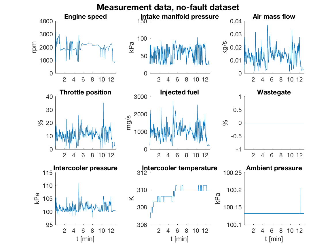
Evaluation on Test Cell Measurements
To illustrate performance on measurement data we consider only 4 of
the 11 faults; faults in the air-flow sensor fy_waf, the intake
manifold pressure sensor fyp_im, the intercooler pressure
sensor fyp_ic, and the intercooler temperature sensor
fyT_ic. Measurement data were collected for the fault free and
4 faulty cases, then in total 5 data sets, during a 12 minute long EPA highway
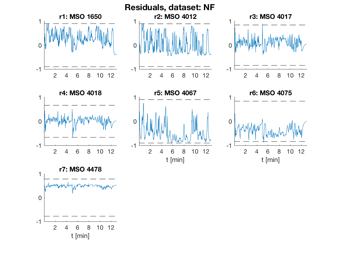
fuel economy test cycle. Sample measurements from the fault free case are
Out of the 728 residuals only a few is needed for isolating between
the 4 faults and using a data-driven test selection procedure not
described here, 7 residuals were in the end chosen for this
illustration. Using class methods FSM and
IsolabilityAnalysisArrs, the fault signature matrix and the
isolability matrix of the selected 7 residuals are
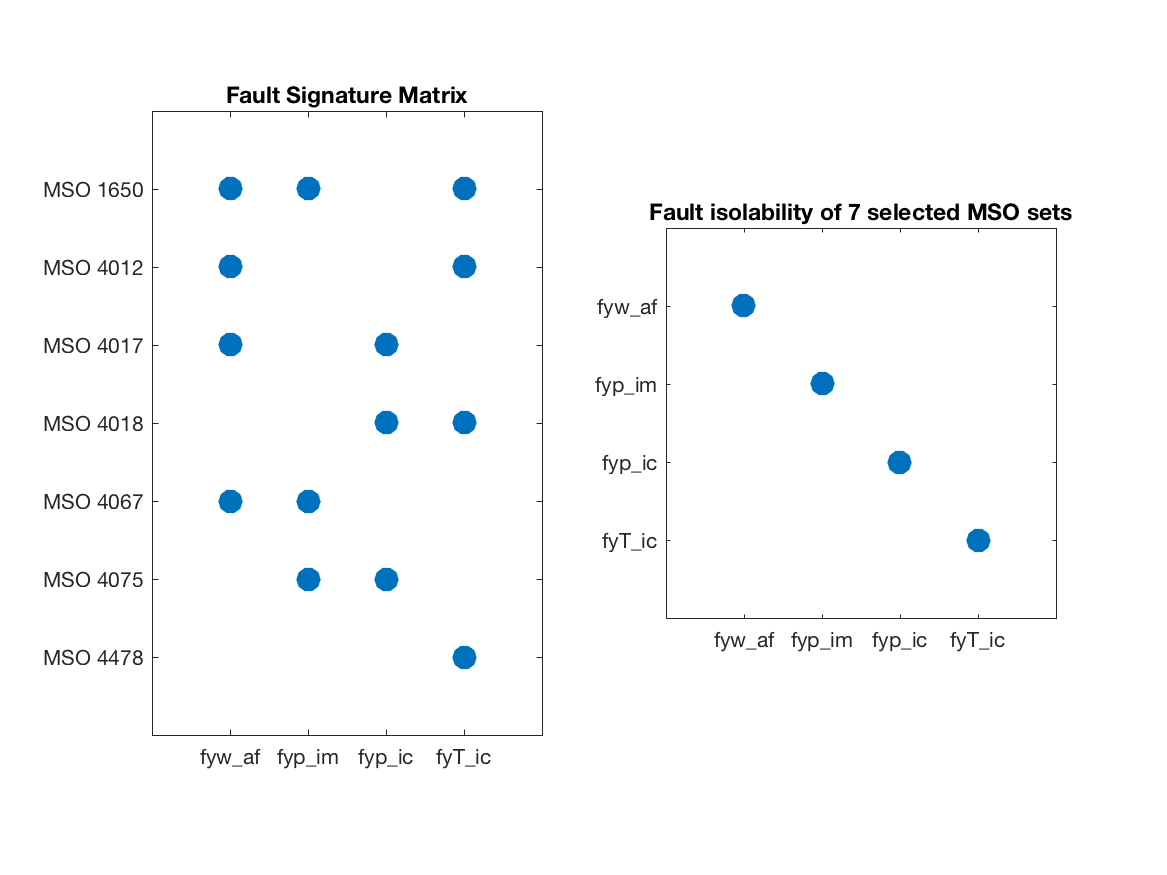
As can be seen, all single faults are structurally isolable.
Running residual generators
The generated code for the 7 residuals are run on the 5 data sets and the residuals in the fault free case are shown in the plot below where the dashed lines correspond to thresholds selected to achieve a 1% false alarm probability.
The generated code from last section is run using the single Matlab call
r = ResGen_1650_74(z, state_init, params, Ts); where z is a matrix with the measurements, the struct state_init
gives the initial state, params the model parameters, and
Ts the sampling time. It takes about 0.55 seconds to evaluate a
residual for 12 minutes of 1kHz sampled data on a 2016 Macbook Pro
which corresponds to about 1500 times faster than real-time.
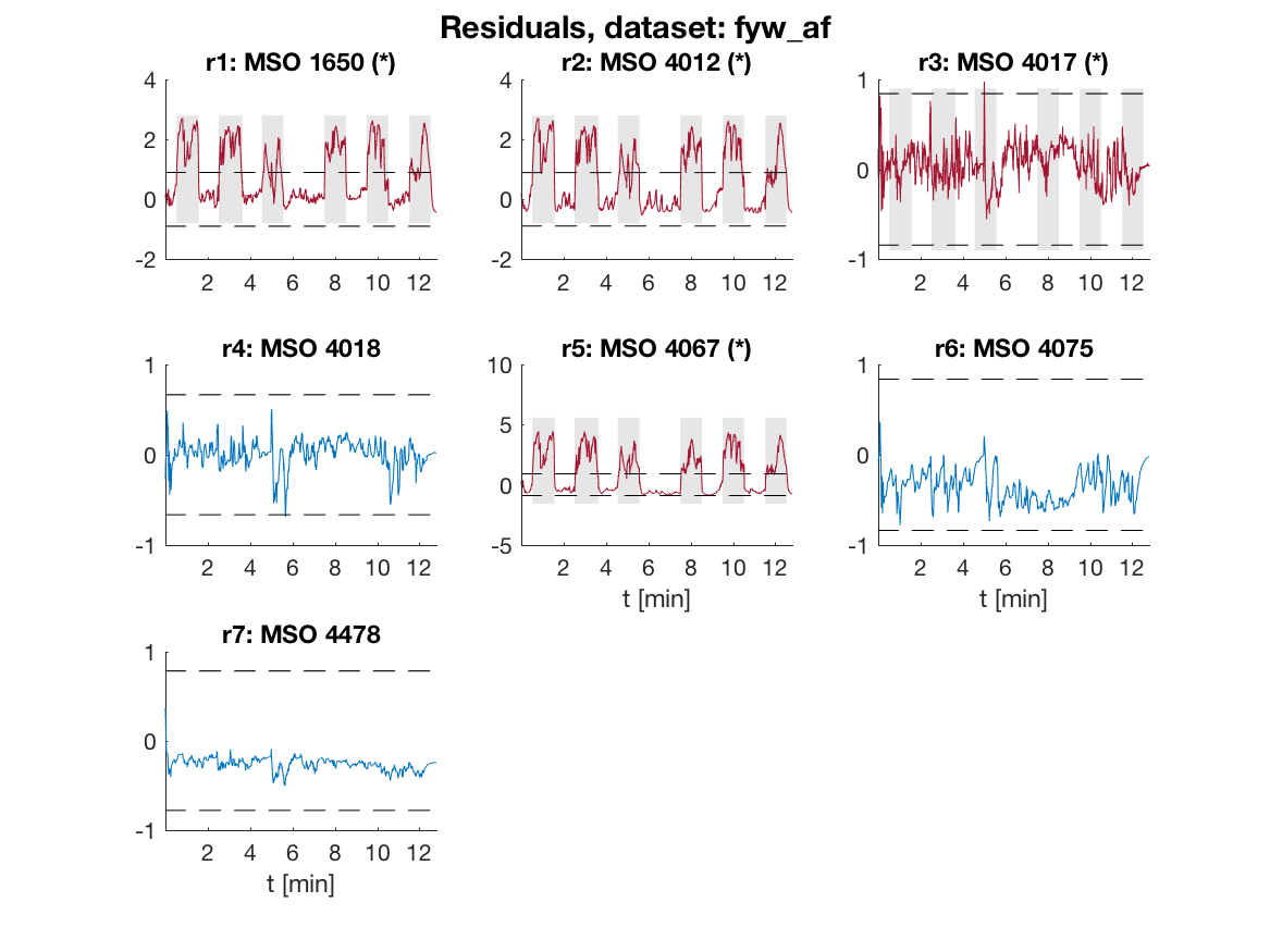
The residuals for data with a fault in the air-flow sensor are
Fault Isolation Performance
According to the fault signature matrix above, the
red colored residuals should be sensitive to the air-flow sensor fault
but not the blue colored residuals. The fault is present during the
gray shaded intervals, i.e., the fault is injected intermittently. The
blue colored residuals are not sensitive to the fault as expected and
residuals 1, 2, and 5 are above the dashed thresholds when the fault is
present. Residual 3 should be sensitive to this fault but the fault to
noise ratio is apparently too low for this fault, but is selected for
its ability to detect fault fyp_ic.
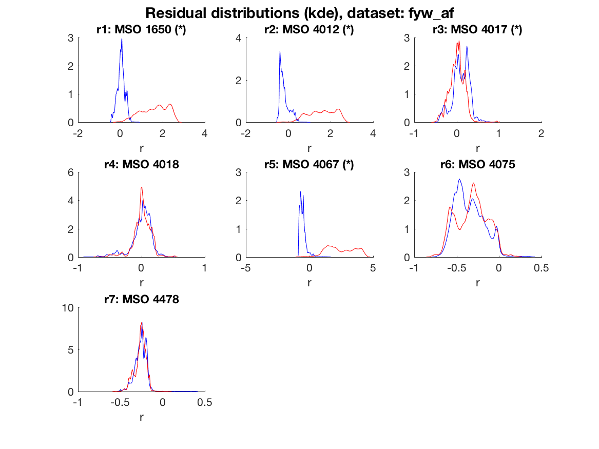
The figure below shows in blue the distributions of the residuals in the fault free case and in red the distributions of the residuals for an air-flow sensor fault. It is clear that residuals 1, 2, and 5 are good at detecting this fault since the residual distributions change significantly.
Given the residuals and thresholds, the consistency based diagnosis candidates as a function of time, in the case of an air mass-flow sensor fault, are
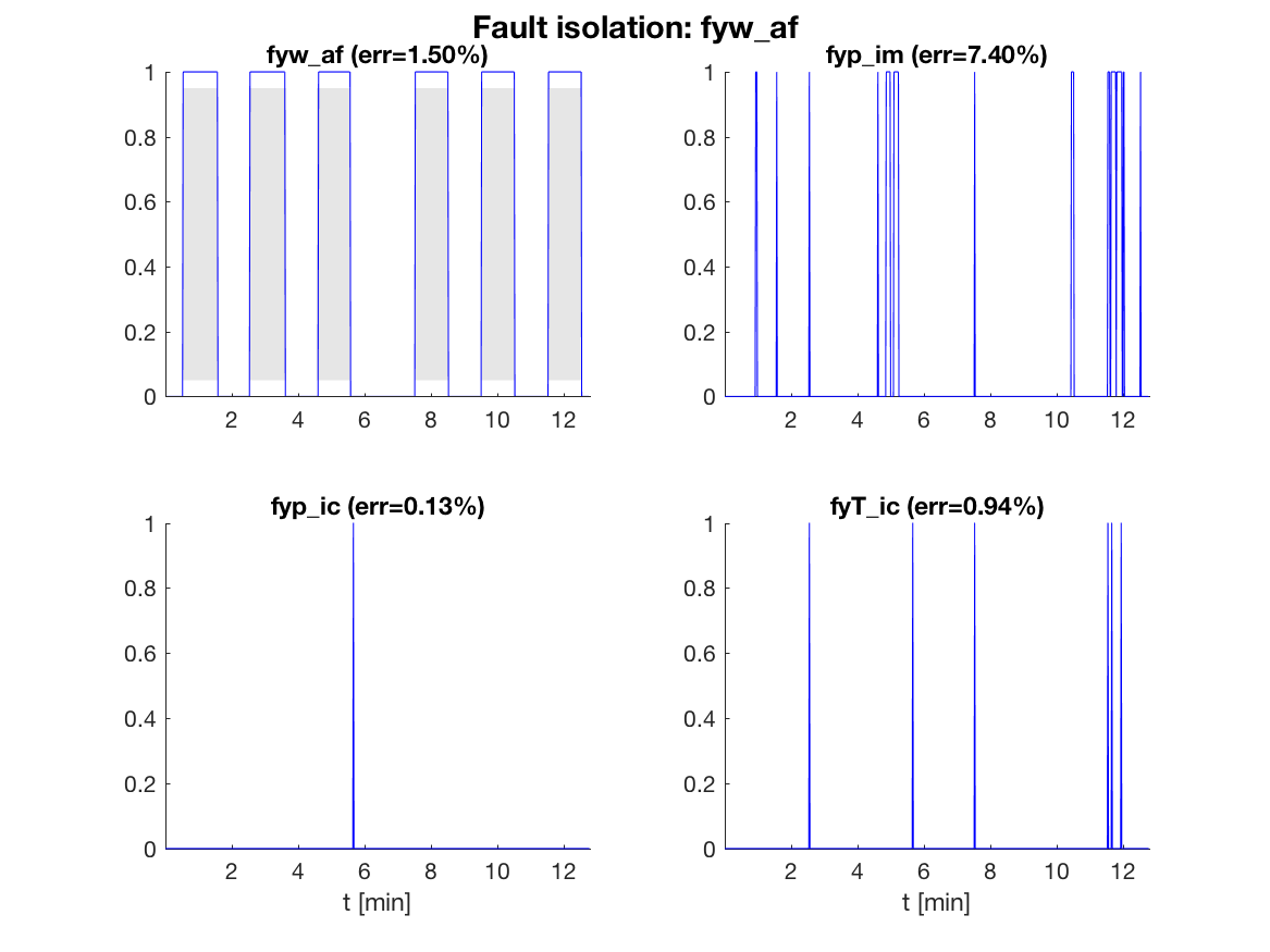
In the figure, a 1 means that the fault is a diagnosis and a
0 that it is not. The percentage of time where there is an isolation
error is shown above each plot. Here, no post-processing is performed,
and the error can be improved by post-filtering or applying adaptive
thresholds, maybe at the cost of a delayed detection.
It is clear that the fault isolation reliably indicates the correct
fault fyw_af and isolates reliably from fyp_ic and
fyT_ic but has a little more difficulty isolating from fault
fyp_im.
To summarize the performance of the generated diagnosis system, the confusion matrix is illustrated using a 3D-plot
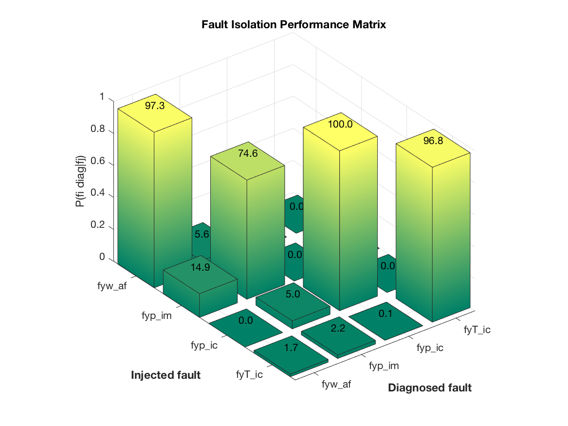
Here, the probability of correct isolation is plotted, and a perfect system
would correspond to a diagonal with probability 1. It is clear from the figure
that faults fyw_af, fyp_ic, and fyT_ic can be reliably isolated. Fault fyp_im
however can be reliably detected but is sometimes difficult to isolate from fyw_af.