Basic usage and introduction to the Python package

This tutorial illustrates basic usage of the python package, gives pointer to some examples, and shows how to install everything on a Linux/MacOS/Windows system.

Outline

1. Induction motor example
   • Modelling
   • Model information, basic plotting, and MSO/MTES
   • Isolability analysis
   • Code generation and residual generation
2. Some more examples
3. Installation

Induction motor example

To illustrate the functionality, a small induction motor example will be used where the model equations are borrowed from the paper Aguilera, F., et al. “Current-sensor fault detection and isolation for induction-motor drives using a geometric approach”, Control Engineering Practice 53 (2016): 35-46.

Modelling

For reference, the equations are given below

There are also three measurement equations, where the two current sensors have modeled faults as

The modeling part is where the main differences between Python and Matlab versions are. This is due to that SymPy is used instead of the symbolic toolbox in Matlab. Therefore, let’s import the toolbox and sympy

import faultdiagnosistoolbox as fdt
import sympy as sym

Now, we define the model as a python dictionary with keys

• type - type of model, here we are definic a model using symbolic expressions
• x - list of unknown variables in the model
• f - list of fault variables
• z- list of known variables
• rels - list of model equations
• parameters - list of parameters (optional) For the induction motor model, this corresponds to

model_def = {'type': 'Symbolic',
             'x': ['i_a', 'i_b', 'lambda_a', 'lambda_b', 
                   'w', 'di_a', 'di_b', 'dlambda_a', 
                   'dlambda_b', 'dw', 'q_a', 'q_b', 'Tl'],
             'f': ['f_a', 'f_b'], 
             'z': ['u_a', 'u_b', 'y1', 'y2', 'y3'],
             'parameters': ['a', 'b', 'c', 'd', 'L_M',
                            'k', 'c_f', 'c_t']}

# Make symbolic objects of all variables/parameters before writing down equations.
sym.var(model_def['x'])
sym.var(model_def['f'])
sym.var(model_def['z'])
sym.var(model_def['parameters'])

model_def['rels'] = [
  -q_a + w*lambda_a,
  -q_b + w*lambda_b, 
  -di_a + -a*i_a + b*c*lambda_a + b*q_b+d*u_a,
  -di_b + -a*i_b + b*c*lambda_b + b*q_a+d*u_b,
  -dlambda_a + L_M*c*i_a - c*lambda_a-q_b, 
  -dlambda_b + L_M*c*i_b - c*lambda_b-q_a, 
  -dw + -k*c_f*w + k*c_t*(i_a*lambda_b - i_b*lambda_a) - k*Tl,
  fdt.DiffConstraint('di_a','i_a'),
  fdt.DiffConstraint('di_b','i_b'),
  fdt.DiffConstraint('dlambda_a','lambda_a'),
  fdt.DiffConstraint('dlambda_b','lambda_b'),
  fdt.DiffConstraint('dw','w'),
  -y1 + i_a + f_a,
  -y2 + i_b + f_b,
  -y3 + w]

Now, the DiagnosisModel object can be created as

model = fdt.DiagnosisModel(model_def, name ='Induction motor')

and the API is very close to the Matlab version as described in the documentation.

Model information, basic plotting, and MSO/MTES

As before, to display model information use the Lint class method

model.Lint()

which gives

Model: Induction motor
  Type:Symbolic, dynamic
  Variables and equations
    13 unknown variables
    5 known variables
    2 fault variables
    15 equations, including 5 differential constraints
  Degree of redundancy: 2
  Degree of redundancy of MTES set: 1
  Model validation finished with 0 errors and 0 warnings.

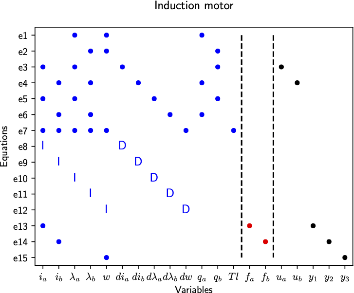
The degree of redundancy is 2 in the model since there are 3 output sensors and 1 unknown input to the system, the load torque Tl. To plot the model structure, use the PlotModel method as

# Plot model
model.PlotModel()

which gives the figure

Computing the set of MSO and MTES sets is done as below

# Find set of MSOS and MTES
msos = model.MSO()
mtes = model.MTES()
print(f"Found {len(msos)} MSO sets and {len(mtes)} MTES sets.")

# Check observability and low index for MSO sets
oi_mso = [model.IsObservable(m_i) for m_i in msos]
li_mso = [model.IsLowIndex(m_i) for m_i in msos]
print(f'Out of {len(msos)} MSO sets, {sum(oi_mso)} observable, {sum(li_mso)} low (structural) differential index')

# Check observability and low index for MTES sets
oi_mtes = [model.IsObservable(m_i) for m_i in mtes]
li_mtes = [model.IsLowIndex(m_i) for m_i in mtes]
print(f'Out of {len(mtes)} MTES sets, {sum(oi_mtes)} observable, {sum(li_mtes)} low (structural) differential index')

and the code outputs

Found 9 MSO sets and 2 MTES sets.
Out of 9 MSO sets, 9 observable, 4 low (structural) differential index
Out of 2 MTES sets, 2 observable, 2 low (structural) differential index

Isolability analysis

To plot the isolability properties of the model under mixed casaliyu asssumption

# Isolability analysis
model.IsolabilityAnalysis(plot=True, causality='mixed')

and to examine in more detail, the Dulmage-Mendelsohn decomposition with a canonical form of the overdetermined subsystem is plotted by

model.PlotDM(fault=True, eqclass=True)

which gives the figure

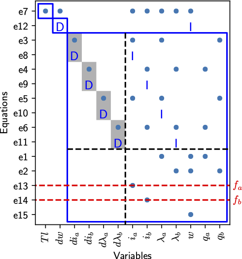
For more details on the canonical decomposition of the overdetermined part, see Mattias Krysander, Jan Åslund, and Mattias Nyberg, “An Efficient Algorithm for Finding Minimal Over-constrained Sub-systems for Model-based Diagnosis”. IEEE Transactions on Systems, Man, and Cybernetics – Part A: Systems and Humans, 38(1), 2008.

Code generation and residual generation

To wrap up this example, let us use one of the MTES sets and generate C++-code for a residual generator. First, let’s see which redundant equation that can be used for integral causality residual generation using the MSOCausalitySweep class method

model.MSOCausalitySweep(mtes[0])

This outputs

['mixed', 'mixed', 'mixed', 'mixed', 'mixed', 'mixed', 'mixed', 'int', 'mixed', 'mixed', 'int', 'mixed']

and thus the 11:th element in the first MTES can be used. The 11:th element correspond to the second measurement equation

red_eq = mtes[0][10]
model.syme[red_eq]
Out[50]: Eq(f_b + i_b - y2, 0)

Now, get the rest of the equations to form the exactly determined set of equations and compute a mathing using the Matching class method

M0 = [e for e in mtes[0] if e != red_eq]
Gamma = model.Matching(M0)

Now, all is set to generate the residual generator code using the SeqResGen class method

model.SeqResGen(Gamma, red_eq, 'ResGen', batch=True, language='C')

which generate files ResGen.cc and ResGen_setup.py. Have a look at the ResGen_core() function in the generated C++-file and you’ll se how things work. The generated code can now be compiled by executing

python ResGen_setup.py build_ext --inplace

in a terminal.

More examples

In the distribution, there are a few more examples included. To find where pip puts everything, run

fdt.__path__

and have a look in the examples sub-folder.

Installation

The package needs Python version 3.6 or newer, check which version you have installed with

python3 --version

Now, create a virtual environment, don’t install into the system wide python installation. You can do this as (only needed once) with

python3 -m venv env

and then activate the environment as

source ./env/bin/activate  # Linux/MacOS

in MacOS/Linux or if you’re on a Windows machine

.\env\Scripts\activate  # Windows

Always a good idea to upgrade the package manager pip before continuing

pip install --upgrade pip

Then, install the toolbox

pip install faultdiagnosistoolbox

and that is that.