Random Forest Test Selection

This tutorial describes how a machine learning classifier, random forest, can be used in a data driven approach to residual selection.

The method is described in detail in the publication “Residual Selection for Consistency Based Diagnosis Using Machine Learning Models” published at IFAC Safeprocess 2018 in Warszaw, Poland. Find the full paper at https://doi.org/10.1016/j.ifacol.2018.09.547.

All code and data to generate the plots below are included in full in the in the provided examples suite in the toolbox distribution, in the examples/TestSelection directory.

Background

A common architecture of model-based diagnosis systems is to use a set of residuals to detect and isolate faults. In many cases there are more possible candidate residuals than needed for detection and single fault isolation and key sources of varying performance in the candidate residuals are model errors and noise. This tutorial demonstrates an approach that combines a machine learning model, random forest, with diagnosis specific performance specifications to select a high performing subset of residuals. The approach is illustrated using an industrial use case, an automotive engine, and it is shown how the trade-off between diagnosis performance and the number of residuals easily can be controlled.

The use case is an automotive engine where model-based techniques has been used to
generate residuals. See the use-case for full details how the residuals are generated; the only difference here is that more fault modes are considered. In this tutorial, the residuals have been generated and saved in a file so there is no need to generate the data.

Problem formulation

The problem to be solved is to select a subset of the 42 residuals that have been generated, preferably a small subset, that have similar diagnosability performance as the full set of 42 residuals.

The system and residuals

In the dataset there are 42 generated residuals for the no-fault mode and 7 different fault modes. Below are 7 of the residuals plotted for the 7+1 different fault modes.

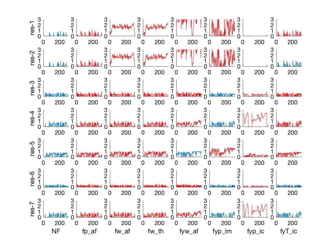
The red residuals correspond to cases where the residual should, structurally, raise an alarm and the blue where there should be no alarm. All residuals are normalized such that a threshold of 1 correspond to a fixed false-alarm probability.

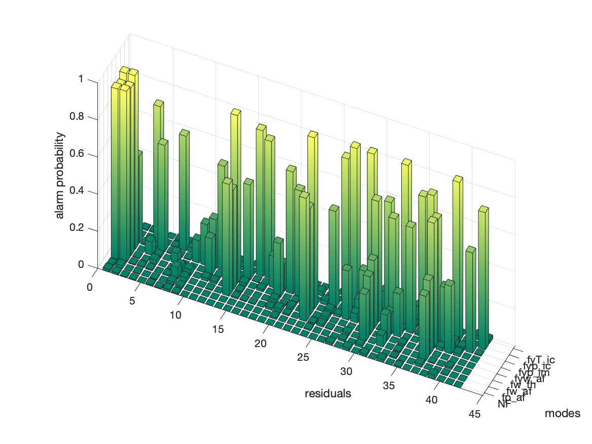
It is clear that not all residuals that should raise an alarm, i.e., the red residuals, react and therefore this information can be of use to select residuals. The figure below show, for each residual, what is the probability of an alarm

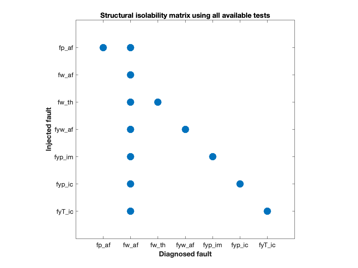The ideal fault isolation performance of the 42 generated residuals are summarized in the structural fault isolation matrix. From this matrix it is clear that, even if the model is perfect, it is not possible to isolate the fault fw_af from the others, although it can be detected. This information is important to take into consideration when looking for a subset of residuals that can achieve diagnosability performance that is similar to the full set of 42 residuals.

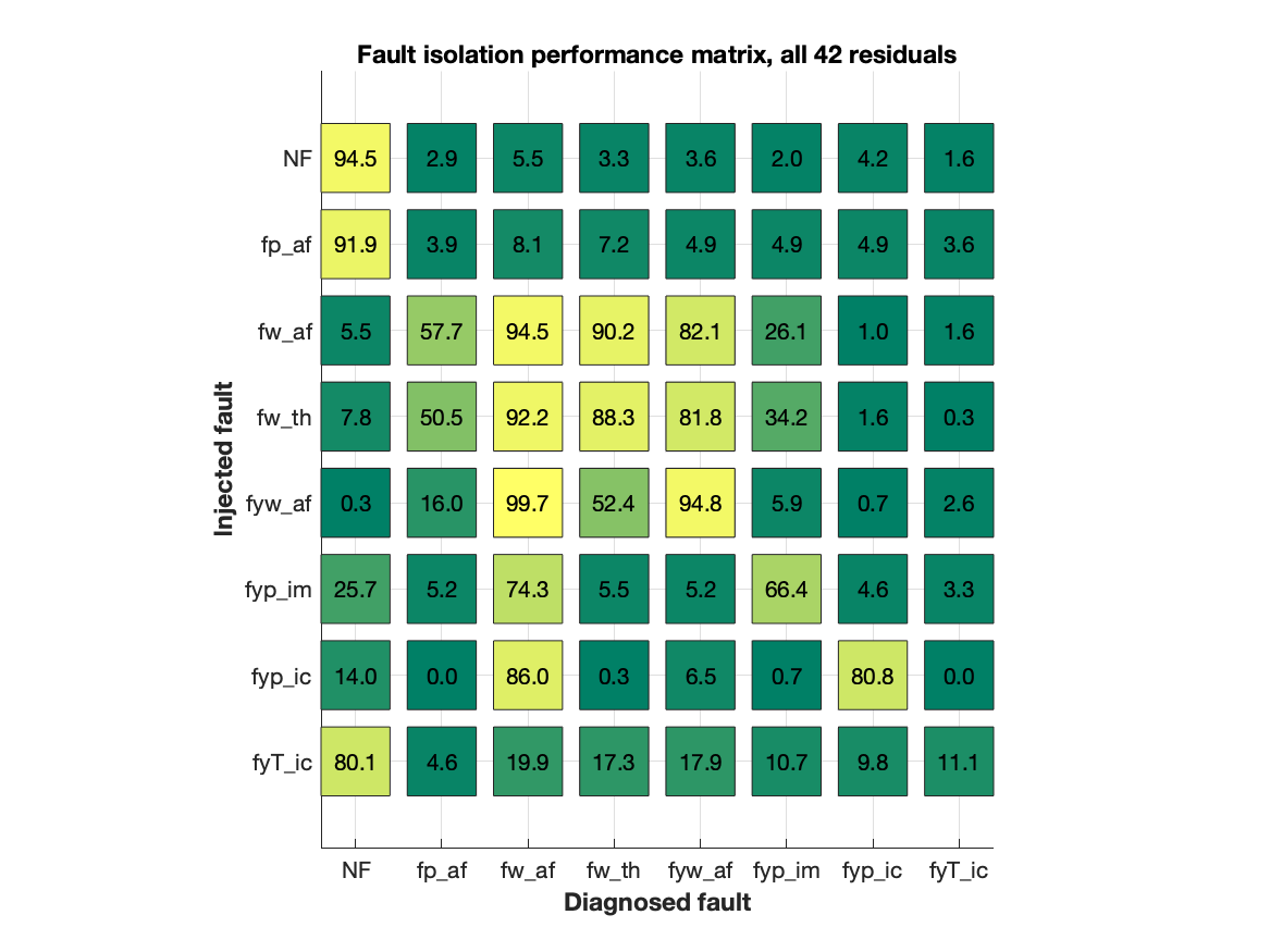
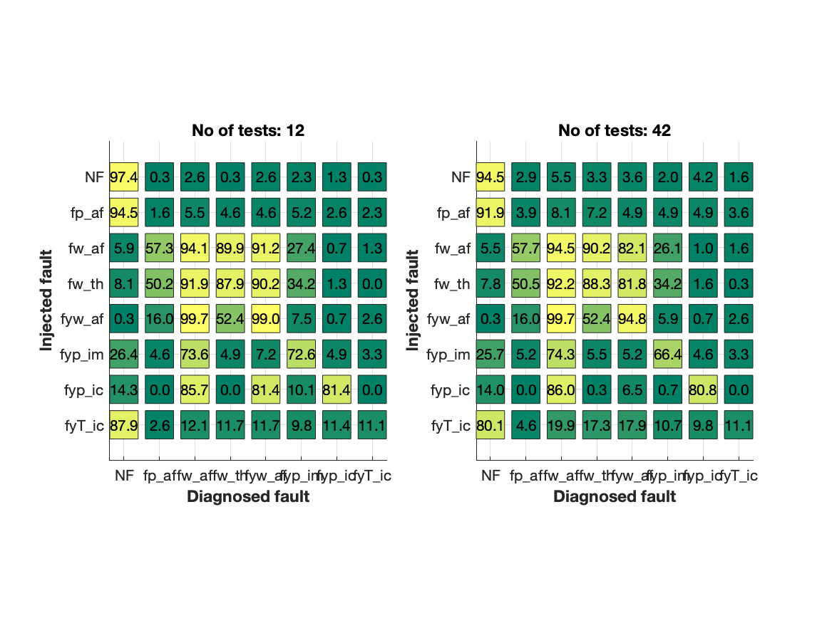
Residual performance of the full set of residuals

The confusion matrix below shows the performance of the full set of 42 residuals. This shows the probability that a fault is a diagnosis, given an injected fault. In an ideal case, the confusion matrix should be 100% all along the diagonal. Clearly, as indicated by the structural fault isolation matrix above, this is not possible.

The figure is generated using the code

[~, C] = DiagnosesAndConfusionMatrix(thdata);
PlotConfusionMatrix(C, thdata.modes);
title('Fault isolation performance matrix, all 42 residuals');

where thdata is a Matlab structure with the data, the fault signature matrix, and definition of fault modes. This performance is the goal, i.e., choose a subset of residuals such that the confusion matrix is as similar as possible to the confusion matrix above.

Residual selection approach

The Random Forest test selection algorithm is called as

[result, C, rf, Crf, oobErr] = RandomForestTestSelection(thdata, 200);

where the parameter 200 indicates how many decision trees to be built in the random forest approach. The outputs architecture

• result - A structure with the result of the selection approach. The structure have the fields
  • sortidx: A sorted list of indices to residuals with the most important residuals first.
  • pfa : Performance curve for the false alarm probability
  • pmd : Performace curve for missed detection
  • pfi : Performance curve for fault isolation
  • pmfi : Maximal isolation performance per fault mode
  • residualimportance : List of relative residual importance.
• C - A confusion matrix when computing consistency based diagnoses using all residuals.
• rf - The random forest object
• Crf - The confusion matrix for the random forest classifier.
• oobErr - Out-of-bag error rate

After building the random forest, a sorted list of residual/test importance can be plotted with the code

plot(result.residualimportance(result.sortidx))
xticks(1:length(result.sortidx))
title('Out-of-Bag Permuted Predictor Importance Estimates');
ylabel('Estimates');
xlabel('Predictors')

generating the plot

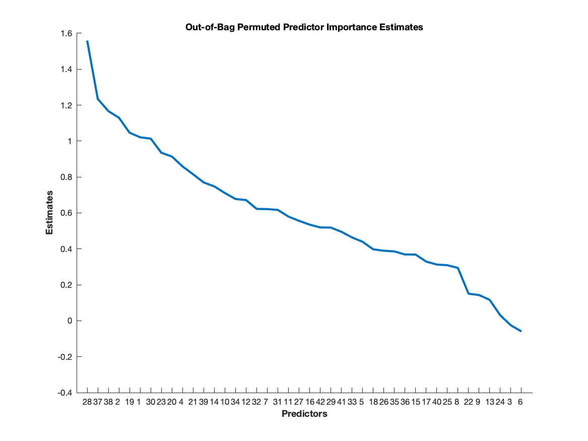
This plot indicates the order in which residuals should be selected. To determine how many to select, the performance curves computed is useful. The code

plot([result.pmd, result.pfa, result.pfi])
legend('Missed detection probability', 'False alarm probability', ...
       'Fault isolation errors')
xlabel('Number of selected residuals')
ylabel('Probability')

generates the plot

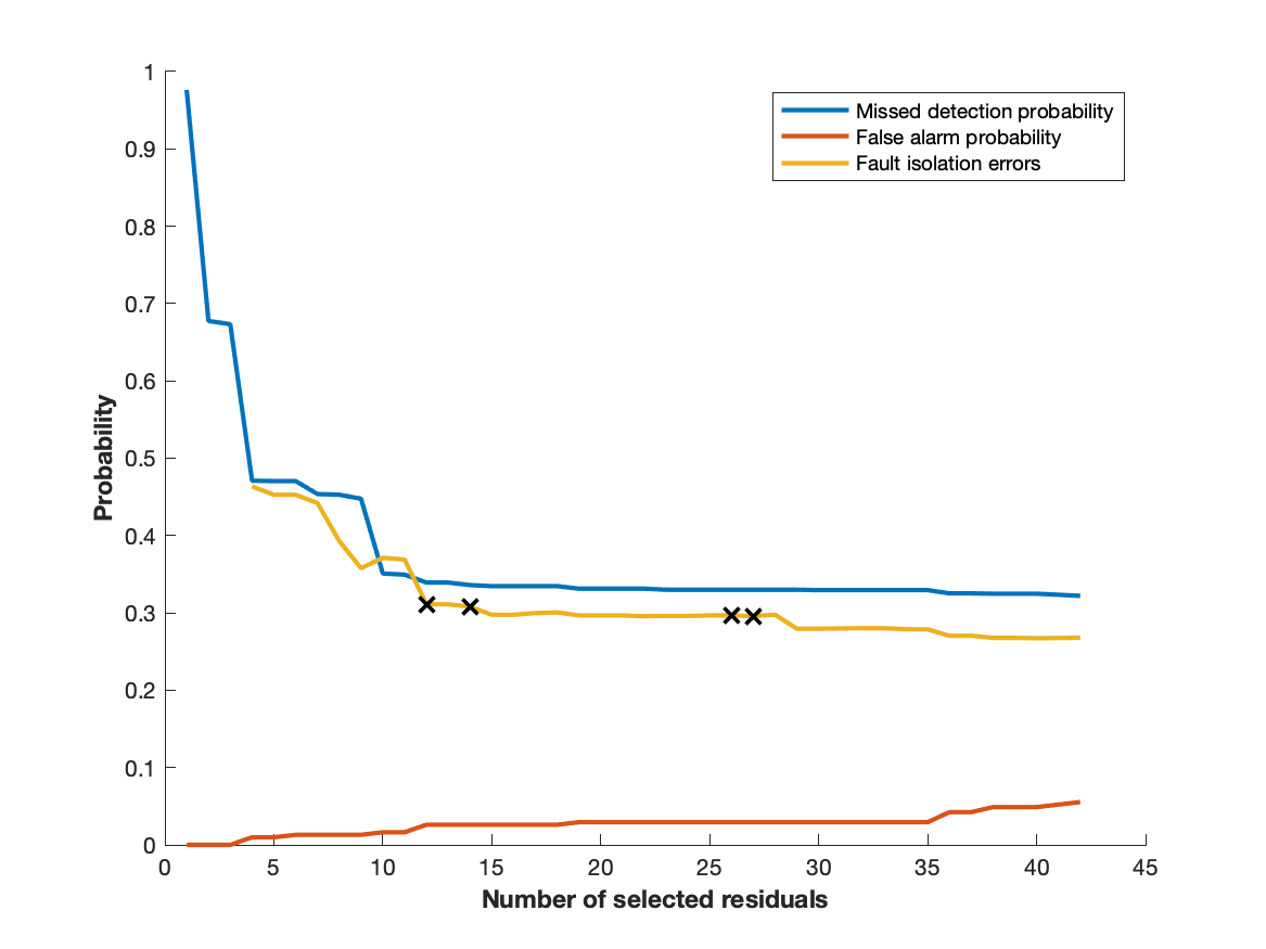
which indicates that full performance is acheived after approximately 12 selected residuals. Then, selecting 12 residuals in the order according to the ranking above gives a confusion matrix that compares with the confusion matrix obtained when using all residuals.

Conclusion

The illustrated approach, a procedure with little tuning, the number of residuals was reduced from 42 to 12 and still achieving almost identical diagnosis performance.