Defining a symbolic dynamic model

This tutorial describes how to define a symbolic model with dynamic constraints.

Click here for the full script for this tutorial.

Again, as in a previous tutorial an idealized model of an electric motor will be used 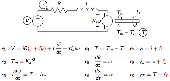where V is voltage, i current, Tm motor torque, Tl load torque, omega rotational speed, theta motor angle. There are four considered faults, three sensor faults and a change in the internal resistance.

Here the full symbolic model, including dynamic constraints, will be defined. For this, create a model definition with the type

modelDef.type = 'Symbolic';

After that, partition the set of variables in three categories; unknown (x), known (z), and faults (f), and also determine the set of parameters in the model. Since we are considering dynamics, introduce variables also for the derivatives. Then,

modelDef.x = {'dI','dw','dtheta', 'I','w','theta','alpha','T','Tm','Tl'};
modelDef.f = {'fR','fi','fw','fT'};
modelDef.z = {'V','yi','yw','yd'};
modelDef.parameters = {'Ka','b','R','J','L'};

The next step is to define symbolic expressions for all model variables so that the symbolic toolbox can manage them.

syms(modelDef.x{:})
syms(modelDef.f{:})
syms(modelDef.z{:})
syms(modelDef.parameters{:})

Now, we can state the model equations directly as

modelDef.rels = {...
  V == I*(R+fR) + L*dI + Ka*I*w,...  % e1
  Tm == Ka*I^2, ...                  % e2
  J*dw == T-b*w, ...                 % e3
  T == Tm-Tl, ...                    % e4
  dtheta == w, ...                   % e5
  dw == alpha, ...                   % e6
  yi == I + fi, ...                  % e7
  yw == w + fw, ...                  % e8
  yd == T + fT, ...                  % e9
  DiffConstraint('dI','I'),...       % e10
  DiffConstraint('dw','w'),...       % e11
  DiffConstraint('dtheta','theta')}; % e12

Note especially how the differential constraints e10, e11, and e12 are defined. Also, you can clean up the workspace to keep it from cluttering by

clear( modelDef.x{:} )
clear( modelDef.f{:} )
clear( modelDef.z{:} )
clear( modelDef.parameters{:} )

Now, the model definition is complete and we can create the model object and give it a name as before

model = DiagnosisModel( modelDef );
model.name = 'Electric motor';

With the model object defined, print some basic model information using the class method Lint

>> model.Lint()
Model: Electric motor

  Type: Symbolic, dynamic

  Variables and equations
    10 unknown variables
    4 known variables
    4 fault variables
    12 equations, including 3 differential constraints

  Degree of redundancy: 2
  Degree of redundancy of MTES set: 1

  Model validation finished with 0 errors and 0 warnings.

The model structure is automatically inferred from the analytical expressions. And to graphically plot the model structure, use the PlotModel class method

model.PlotModel()

which produces the figure 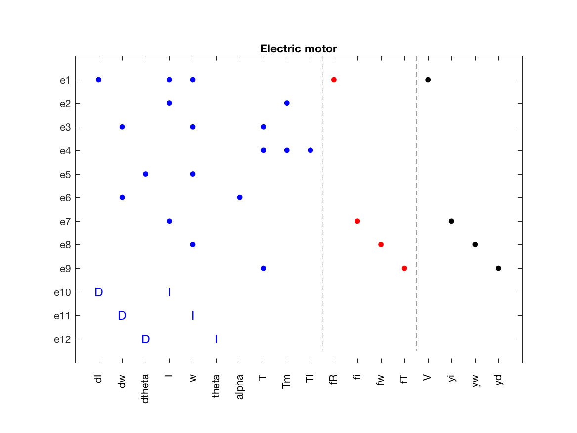Here, the dynamic constraints can be seen as I and D edges in the incidence matrix.