Isolability analysis and sensor placement

This tutorial describes how to perform basic isolability analysis for a model and sensor placement analysis.

Click here for the full script for this tutorial.

Again, as in a previous tutorial an idealized model of an electric motor will be used 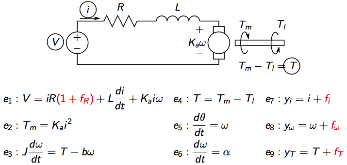where V is voltage, i current, Tm motor torque, Tl load torque, omega rotational speed, theta motor angle. There are four considered faults, three sensor faults and a change in the internal resistance.

Follow the previous tutorial to define the model. After the model has been defined, use the class method Lint to show basic model information

>> model.Lint()
Model: Electric motor

  Type: Symbolic, dynamic

  Variables and equations
    10 unknown variables
    4 known variables
    4 fault variables
    12 equations, including 3 differential constraints

  Degree of redundancy: 2
  Degree of redundancy of MTES set: 1

  Model validation finished with 0 errors and 0 warnings.

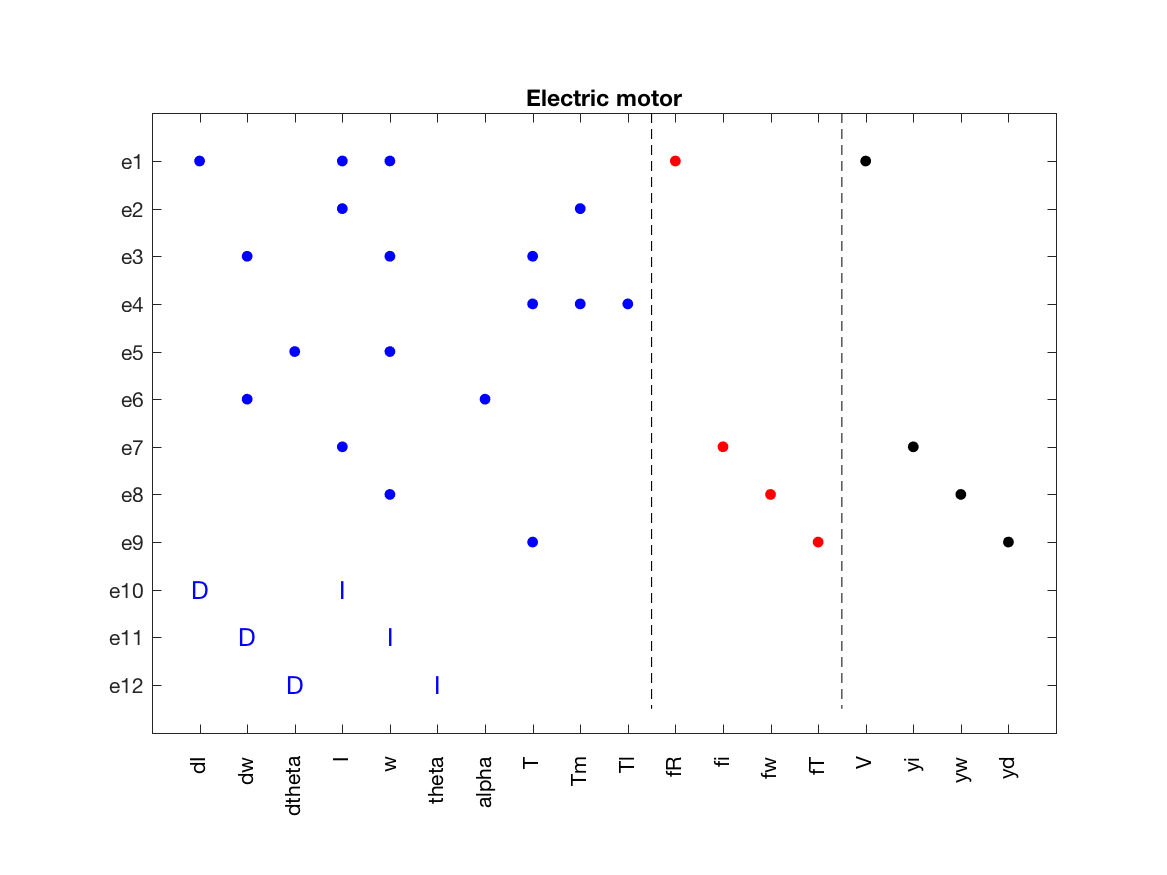
and the model structure can be shown using the PlotModel class method

model.PlotModel()

which produces the figure

Isolability analysis

The model is over-constrained, i.e., more equations than unknown due to the three measurement equations already included. This means that there are redundancy in the model and there is a possibility to create residuals for fault detection and fault isolation. Before designing residuals, it is possible to analyze the model and see what diagnosis performance that is ideally possible with the used sensors. This is called _isolability analysis and can be performed using the class method IsolabilityAnalysis` as

model.IsolabilityAnalysis()

which produces the figure

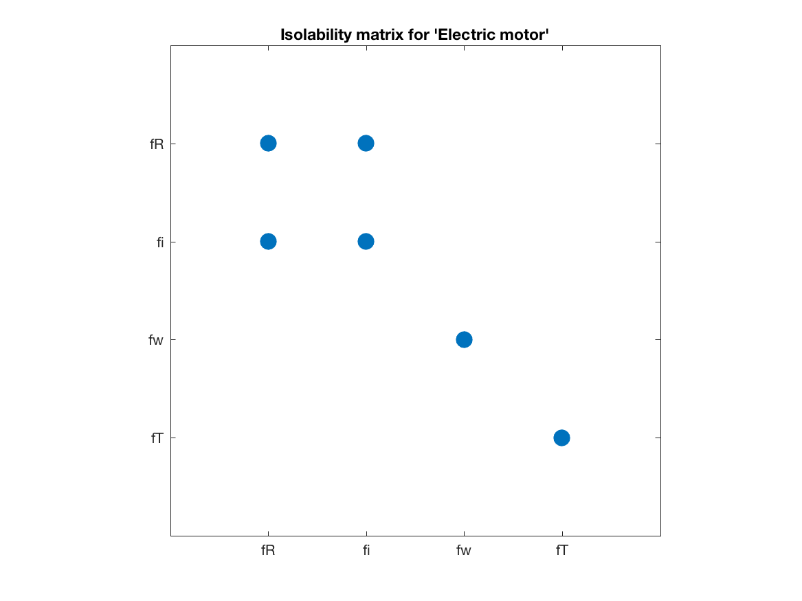
This figure illustrates the isolability matrix, where a dot in position (i,j) indicates that, structurally, fault fi can not be isolated from fault fj. The ideal performance is this a diagonal matrix. Here it is clear that all faults can be detected, faults fw and fT can be uniquely isolated, and faults fR and fi can be isolated from the other two but can not be isolated from each other.

Sensor placement for full isolability

Assume we are considering adding a sensor to be able to achieve ideal isolability performance, a sensor placement analysis tells us which are possible sensor positions. First, tell the model which are the possible sensor locations, and if any new sensors may become faulty. First, consider the case where all unknowns are possible sensor locations and non may become faulty. This done in Matlab using the class methods PossibleSensorLocations and SensorLocationsWithFaults as

model.PossibleSensorLocations({'I', 'w', 'theta', 'alpha', 'T', 'Tm', 'Tl'});
model.SensorLocationsWithFaults([]); % No new sensors may become faulty

Now, perform the sensor placement analysis using the class method SensorPlacementIsolability as

sens = model.SensorPlacementIsolability();

The variable sens now include all minimal sensor sets that achieves full isolability (if possible). In this case, there are three minimal solutions

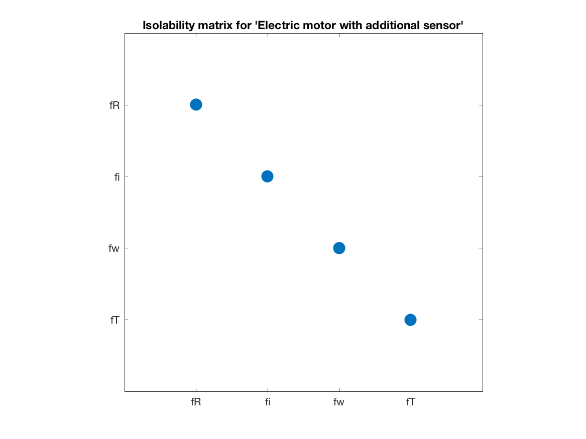
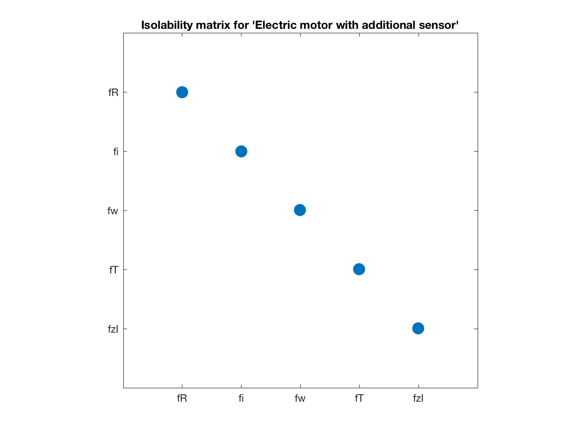
sens = { {'I'}, {'Tm'}, {'Tl'} }

Let’s add the current sensor, and do another isolability analysis to see that we have actually obtained ideal performance

model2 = model.AddSensors( sens{1} );
model2.name = 'Electric motor with additional sensor';
model2.IsolabilityAnalysis()

which produces the isolability matrix

Sensor placement where new sensors may fail

Now, assume that also the new sensors may fail. Tell that to the model and redo the sensor placement analysis

model.PossibleSensorLocations({'I', 'w', 'theta', 'alpha', 'T', 'Tm', 'Tl'});
model.SensorLocationsWithFaults({'I', 'w', 'theta', 'alpha', 'T', 'Tm', 'Tl'});

sens = model.SensorPlacementIsolability();

It turns out that you get the same set of solutions, in this case only this is not a general property. To verify the solution, add the sensor and redo the sensor placement analysis by

model3 = model.AddSensors( sens{1} );
model3.name = 'Electric motor with additional sensor';
model3.IsolabilityAnalysis()

which produces the isolability matrix

which is ideal and note that a new fault has appeard in the analysis, this is the fault in the new sensor.